Making efficient use of your compute resources
The non-trivial matter of optimising compute resources available for your analysis is brought into the spotlight. We discuss when you might benefit from optimising the compute resources available for your analysis as well as how you can achieve this on the Seven Bridges Platform. Examples of effective management of large input files as well as adequate choice of compute resources are provided.
A non-trivial matter
Tools vary a great deal in terms of resource requirements. At one end of the spectrum there are light weight tools like FastQC, which have a low demand for compute resources: 1 CPU and 250 MB of RAM are enough for FastQC to produce a quality control report from a FASTQ file. You could run this tool on your smartphone. The heavyweights at the other end of the spectrum include tools like sequencing read aligners: BWA MEM Bundle will have no problem taking more than 30 CPUs and 30 GB of RAM for a whole genome alignment.
Input size also impacts resource usage. For example, an aligner will require much fewer resources when processing whole exome data, as opposed to whole genome data.
The matter of optimisation is non-trivial. To help you optimise your analysis, the Seven Bridges engineers have exposed features that allow you to control how a job gets executed. It may seem that the gains are small, but they do add up – especially if you are running a single workflow many times.
When should I optimize resource requirements?
If a workflow has one or more tools that accept a list of files as input, it’s advisable to make a rough resource requirement calculation beforehand.
Lists of inputs can vary in length, meaning that the resource requirements set for your workflow could become inappropriate for a particular analysis. If your list of inputs is much smaller than the allocated resources, you will end up paying for compute resources you are not using. Conversely, a very long list of inputs may require more resources than those allocated, leading to bottlenecks in job executions. Jobs that could have been executed in parallel on a more powerful computation instance end up being queued due to lack of resources.
Before starting your calculation, you need to be aware that a job is created every time a tool is executed. If a tool receives a list of files as its input, a separate job will be created for the execution of each file in the list. These jobs can be executed in parallel or in sequence, depending on the compute resources available. We illustrate how to make this rough calculation below with an example on how to choose the best computation instance for your analysis.
The Seven Bridges bioinformaticians have fine-tuned the public apps to make the most of the provisioned compute resources. These settings cover the most common use cases, so if you intend to push the boundaries of the Seven Bridges Public Apps, do check that the compute resources remain appropriate.
How can I optimize for resource requirements?
Resources available to your tool can be optimised by setting the number of parallel instances to be used by the tool and/or by configuring the type of computation instances available.
You can set the maximum number of computation instances that the workflow you are running is allowed to use simultaneously. If the jobs created at one point during the execution of your task do not fit on the specified computation instance, they will be queued and executed by re-using instances as they become available. This ensures that there will be minimal idle time across the entire task.
You can also configure the instance type to be used for your analysis. Depending on the resource requirements of the tool you are using, and whether or not they scatter, you would ideally pick an instance that leaves the least CPU and memory free.
Dealing with large inputs
A “divide and conquer” approach allows tools to process large volumes of data more efficiently by splitting up the input into smaller, independent files.
What was initially a large file is split up into a series of files, meaning that your tool now receives a list of independent files as input. You want each file in this list to be processed separately and in parallel as far as your compute resources permit it.
You can achieve this on the Seven Bridges Platform by enabling scattering. Having this feature enabled for certain tools in your workflow creates a separate job for every element of your list. Jobs are modular units that are then “packed” onto the allocated computation instance(s) for execution. The job packing is orchestrated by the Scheduler, a bespoke Seven Bridges scheduling algorithm which is very good at solving the (in)famous bin packing problem. The Scheduler also assigns and launches compute instances for your tools to execute on.
Thus, using scatter for tools that accept list inputs allows for a more efficient use of compute resources.
Recall that that tools often produce intermediate files during execution. These files are not part of the output and will be deleted before the tool finishes running. However, these intermediate files do take up storage space on the instance while your tool is running. As such, this can deplete the storage space of your instance, which will lead to disk-space overflow errors.
The number and size of the intermediate files varies greatly between tools. Since scattering likely has your tools running several times simultaneously on a single instance, it’s a good idea to factor in the storage space required by intermediate files when using scatter.
Optimizing a whole genome analysis
The Whole Genome Analysis – BWA + GATK 2.3.9-Lite workflow uses scattering when performing local read realignment and variant calling to enable parallelization across the 23 chromosomes.
Parallelization by chromosome is a commonly used method of reducing execution time for a whole genome sequencing analysis.
Let’s run a task using the Whole Genome Analysis – BWA + GATK 2.3.9-Lite workflow with scattering enabled. We can inspect the task stats shown on the Platform to understand how scattering enables efficient use of resources.
The image below shows the section of the GATK workflow we are focusing on, displayed in the Seven Bridges Workflow Editor. The tools we will be discussing are numbered 1 to 6, and the same numbering applies to the task stats image in the second image. The task stats is a graphic timeline representation of the job executions (thin green bars) corresponding to different tools (thick grey bars) in your workflow.
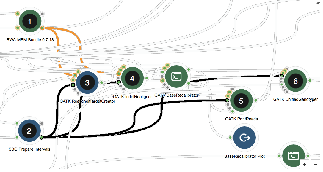
In the workflow, first, global read alignment is performed using BWA-MEM Bundle (1). After this step, we already have a pretty good idea where on the genome reads map to, meaning downstream resource-intensive steps that use the output from this tool (orange connections) can be parallelized by chromosome. The SBG Prepare Intervals tool (2) sets up the chromosome-wise input lists for local read alignments (3 and 4), large file manipulation (5), and variant calling (6).
The GATK tools themselves (3-6) play no role in parallelizing by chromosome – this is achieved by using scatter, a feature implemented by the Seven Bridges Platform. Scatter creates a separate job for each input file in the list – in our case, for each of the chromosomes defined as intervals by the SBG Prepare Intervals tool (2). The connections between the tool generating the list of inputs and the tools using scatter are highlighted in black.
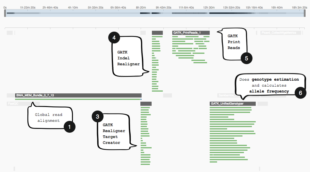
Note how the task stats image above shows only one job (green bar) being executed while BWA-MEM Bundle runs. However, after this has finished, subsequent tools that make use of its output (3-6) will be parallelizing jobs as far as the compute resources on the instancer allow it.
Choosing the best compute instance for your analysis
This example illustrates that it does pay (literally!) to take the time to do a rough resource requirement calculation and set the compute instance for your analysis. If you don’t set an instance for your analysis to be performed on, the Scheduler will try to fit the jobs onto the Platform’s default instance. Because no instance will be best suited for all types of analyses, read below to find out how you can get an idea which instance is best suited for yours.
Let’s say we wrote a tool that processes 23 individual files corresponding to the individual human chromosomes. We have scattering enabled to ensure that all 23 jobs are generated at the same time. Additionally, let’s assume that our tool requires 1 CPU and 4 GB RAM and takes – on average – 45 minutes to complete one job.
If we don’t specify an instance for this tool to be run on, the scheduling algorithm will see that the tool can be run using the default instance – c4.2xlarge with 8 CPU and 15 GB RAM – and will proceed to doing so. By default, only one computation instance is used, so 8 CPUs and 15 GB of RAM is all we have to work with to process the 23 files. The limiting factor is the RAM available on the default instance, which can only allow for 3 jobs – requiring 4 GB of RAM each – to be carried out simultaneously. Hence 3 jobs will be executed in parallel, taking approximately 45 minutes to finish. To execute all of the 23 jobs, they will be organised into 8 batches of maximum 3 jobs each, taking a total of 6 hours to finish (45 min x 8 batches = 360 min). We could reduce the execution time to 45 minutes by increasing the number of instances permitted to run at the same time from 1 to 6 instances; however, in this case we would still be paying for 6 hours of instance time. This costs $2.4. Since we can run at most 3 jobs at a time on each c4.2xlarge instance, we’re only using 3 out of a possible 8 CPUs on each. This ought to make us suspect that a different instance type may provide resources that are a better fit with those we need.
After consulting the list of instances the Seven Bridges Platform has access to on the AWS cloud infrastructure, we can see that a different type of instance could indeed help us achieve better job packing. We choose to use m4.2xlarge – which has 8 CPUs and 32 GB RAM – to run our tool on (see the figure below):
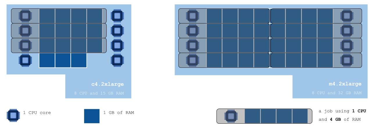
The diagram above shows us how jobs requiring 1 CPU and 4 GB of RAM would be packed onto the default c4.2xlarge instance, versus the instance we chose considering the resource requirements of our analysis. Not taking the time to choose a suitable instance leaves us with 5 idle CPUs and 3 GB of RAM unused – but paid for.The m4.2xlarge would allow for our 23 jobs to be processed in only three batches, taking about two hours and a half in total (45 min x 3 batches = 135 min).
Using the c4.2xlarge instance reduces the instance time required to perform the analysis, and the cost also drops by 45%, to $1.3. The cost of your analysis will likely be reduced overall, but the difference in cost will depend on the hourly rate charged for the chosen instance. Again, we could set the batches to be run in parallel so as to keep the execution time down to 45 minutes.
The table below summaries the execution time and cost of our tool, requiring 1 CPU and 4 GB of RAM, on the compute instances c4.2xlarge (default) and m4.2xlarge (chosen):
| Instance | CPU | RAM [GB] | Cost/hour | Jobs fitted | Batches | Instance time | Total cost |
| c4.2xlarge | 8 | 15 | $0.398 | 3 | 8 | 6 hours (8 x 45 min) | $3.184 |
| m4.2xlarge | 8 | 32 | $0.431 | 8 | 3 | 3 hours (3 x 45 min) | $1.293 |
tl;dr
If your workflow has tools that take lists of files as inputs, try using scatter. This will enable parallelization of tool executions for the elements in your list. If the length of the list is likely to vary significantly, make sure you do a rough resource requirement calculation to check that the available compute resources are still suitable. Another thing to bear in mind is the size of intermediate files, which will take up storage space on your instance while the tool is running.
When bringing your own tools to the Platform, take the time to specify a suitable compute instance for your tool to run on. While the default instance will likely accommodate your analysis, it is not a one-size-fits-all, and you might find that a different instance will reduce the cost of your analysis.