Taxanomic Profiling of Metagenomics Samples
Numerous colonies of different organisms live virtually everywhere on Earth, even in and on our bodies. They are called microbes and we think we know all about them. But do we really?
Actually, the human race knew nothing about microbes before the 17th century. There were some assumptions and hypotheses, but their existence was actually confirmed by Antonie Van Leeuwenhoek and Robert Hooke with the discovery of microscopes. Since then, technology has changed tremendously and now we know that there are organisms from all three domains of life (Archaea, Bacteria, and Eukarya), which are too small to be seen, but all too important for our existence. We learned how to cultivate some of them in the 19th century, and what makes up the genetic basis of their physiology in the last half of the 20th century. Most of the knowledge we obtained about microbes was “laboratory-based”, gathered by observing those culturable microorganisms living in isolation and in artificial conditions. Apart from that, we have very little information about their ecological context or interactions with other organisms from their habitat1.
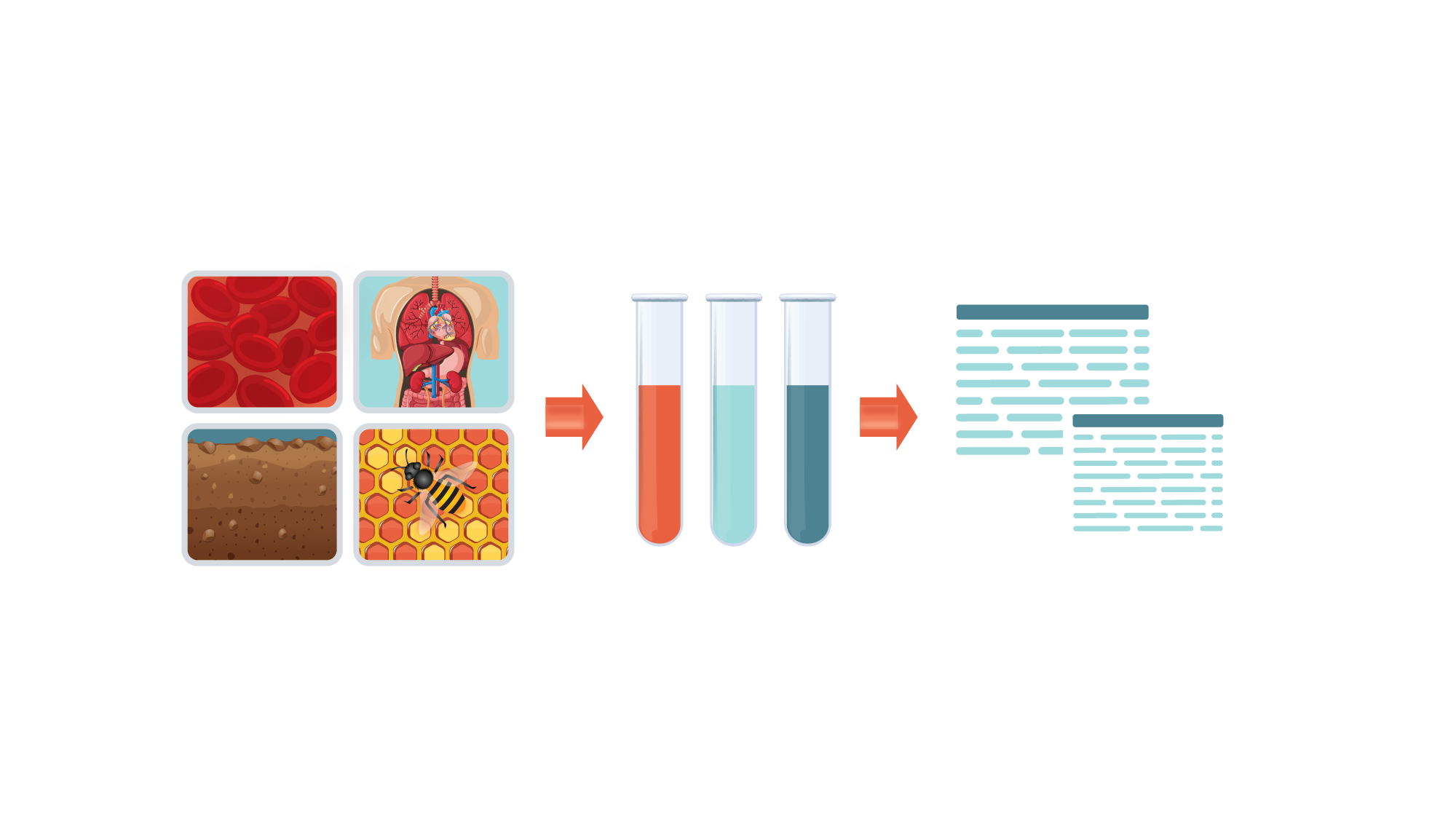
However, metagenomics, the science which explores the mixture of genetic material of microbes directly from their natural environment, is developing fast on the wings of high-throughput sequencing and bioinformatics. Soon, metagenomics will make it possible to investigate the complex communities of these organisms as a whole to reveal which microbes are there, what they do, and what roles microbes play in environmental and physiological processes. The first step would be to identify key features of the microbial ecosystem: which microbes live in different environments, does the composition of the microbial community change with treatment, and can we associate some microbes with certain health conditions and diseases? To find the answers to these and for similar questions, we can use taxonomic profiling of metagenomic samples.
What is taxonomic profiling?
Taxonomic profiling answers the question “Who is there?”, giving us an insight into taxonomic composition of each analyzed sample. Apart from the identification of taxa present in a sample, the relative abundances of organisms are also estimated within this kind of analysis. As a result, the taxonomic profile will contain both a list of detected taxa and their estimated relative abundances as well as the various diversity indices.
Creating a taxonomic profile is not an easy job because metagenomic samples contain genetic material of millions of different organisms from thousands of different species. These molecules are sequenced jointly, so the reads we get from a sequencer could come from any of those organisms. Short read length, high similarity in sequence of genes and genomes, differences in their length, low DNA yield in some cases, or lack of bioinformatics tools and databases all make the problem of microbial identification and taxonomic profiling very challenging.
There are typically two approaches for taxonomic profiling of a metagenomic sample. One uses a single genetic marker (such as 16S rRNA gene for prokaryotes, and 18S or ITS for eukaryotes) and the other one targets the whole genomes of the organisms present in a sample.
The first one, the marker gene based approach2, is limited to detecting only species that have the gene selected, but is usually much cheaper and more widely used. It also cannot distinguish all species, for example Escherichia coli and Shigella spp. share almost identical 16S rRNA gene sequences. When this approach is used, reads are clustered based on their similarity to so-called Operational Taxonomic Units (OTUs). Using the reference database of the marker gene, taxonomic information can be assigned directly to all reads or to aforementioned OTUs, depending on the sequence similarity threshold (typically 95% identity threshold for genus level identification and 97% for species), which will be followed by a diversity analysis.
In the second approach, sequencing reads can originate anywhere from whole microbial genomes. Further analysis can be performed on all of them, or only on a set of reads coming from unique clade-specific marker genes. This method of narrowing the set of reads improves the computational performance while still achieving higher resolution (up to the strain level) 3. On the other hand, there are methods that process reads from whole genomes. Those methods, with advances in computer and data science, have very good performance too4.
Seven Bridges Workflows for Taxonomic profiling of Metagenomic Samples
In order to support metagenomics analyses on the Seven Bridges Platform, we have developed three main workflows (with several additional supporting ones) for taxonomic profiling. They are based on commonly used tools in the bioinformatics and metagenomics research community. For profiling bacterial and archaeal communities from 16S rRNA gene sequences, we have developed QIIME2 16S rRNA Metagenomic Profiling Workflow with QIIME2 tools. Whole metagenome sequences can be analyzed both with Metagenomics WGS analysis – Centrifuge 1.0.3 and Metagenomics WGS analysis – MetaPhlAn 2.0 workflows.
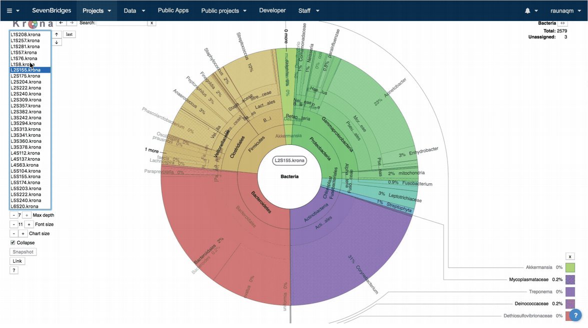
All three workflows will generate, among other workflow specific files, a report with all detected taxa within the samples with their relative abundances. For visualization of the results, we used Krona5 interactive hierarchical graphs (Figure 1), which enable easy browsing through the samples on different taxonomic levels within each sample.
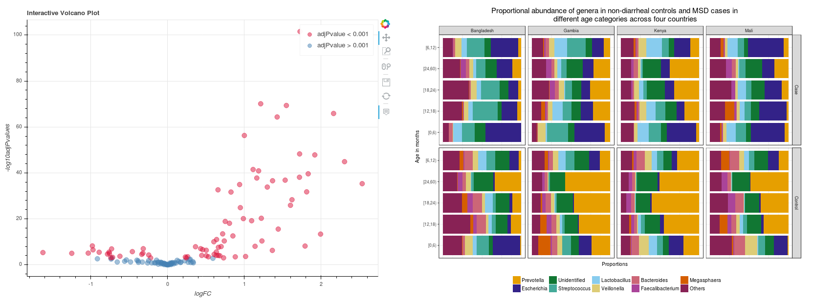
In addition, you can further analyze differential abundances between samples to see whether groups of samples significantly differ in their composition from one another. This analysis is based on the R metagenomeSeq package6 and can be run on the Seven Bridges Platform as an interactive notebook (Figure 2 shows examples of plots from this analysis).
Metagenomics WGS analysis – Centrifuge 1.0.3
Metagenomics Whole Genome Sequencing (WGS) analysis – Centrifuge 1.0.3 is a workflow for analyzing metagenomic samples against a custom reference, allowing researchers to assign reads in their samples to a likely species of origin and quantify each species’ abundance in the sample. This workflow is based on the Centrifuge toolkit, which implements memory-efficient indexing schemes for the classification of microbial sequences based on the FM-index4. The index used for classification of reads is compressed by omitting redundant sequences from highly similar microbial genomes. In this way, the size of the index is reduced, and the search operations become very fast. Another advantage of using Centrifuge is the possibility to create the index from a custom set of microbial genomes in a very convenient and user-friendly way.
For running this workflow on the Seven Bridges Platform, you will need FASTQ files for one or more samples, and Centrifuge index. If you do not have your own index, you can choose one from our Public Repository that best fits your research. You also have an option to create a custom Centrifuge index with our Reference Index Creation workflow.
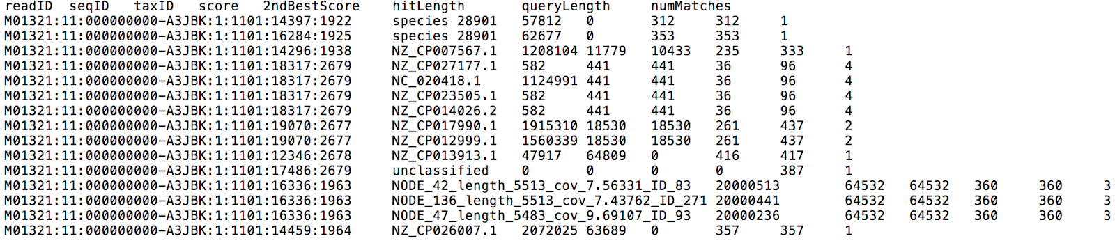
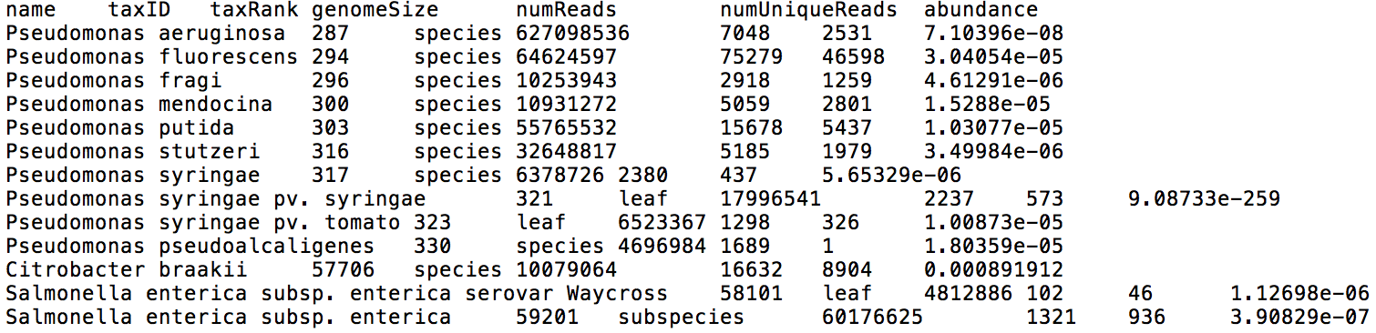
If you input FASTQ files from multiple samples, they will be analyzed in parallel. Centrifuge reports will be output for each sample individually, one with a classification result for each read (Figure 3), and the other one with a list of all taxa found in a sample with their relative abundances (Figure 4).
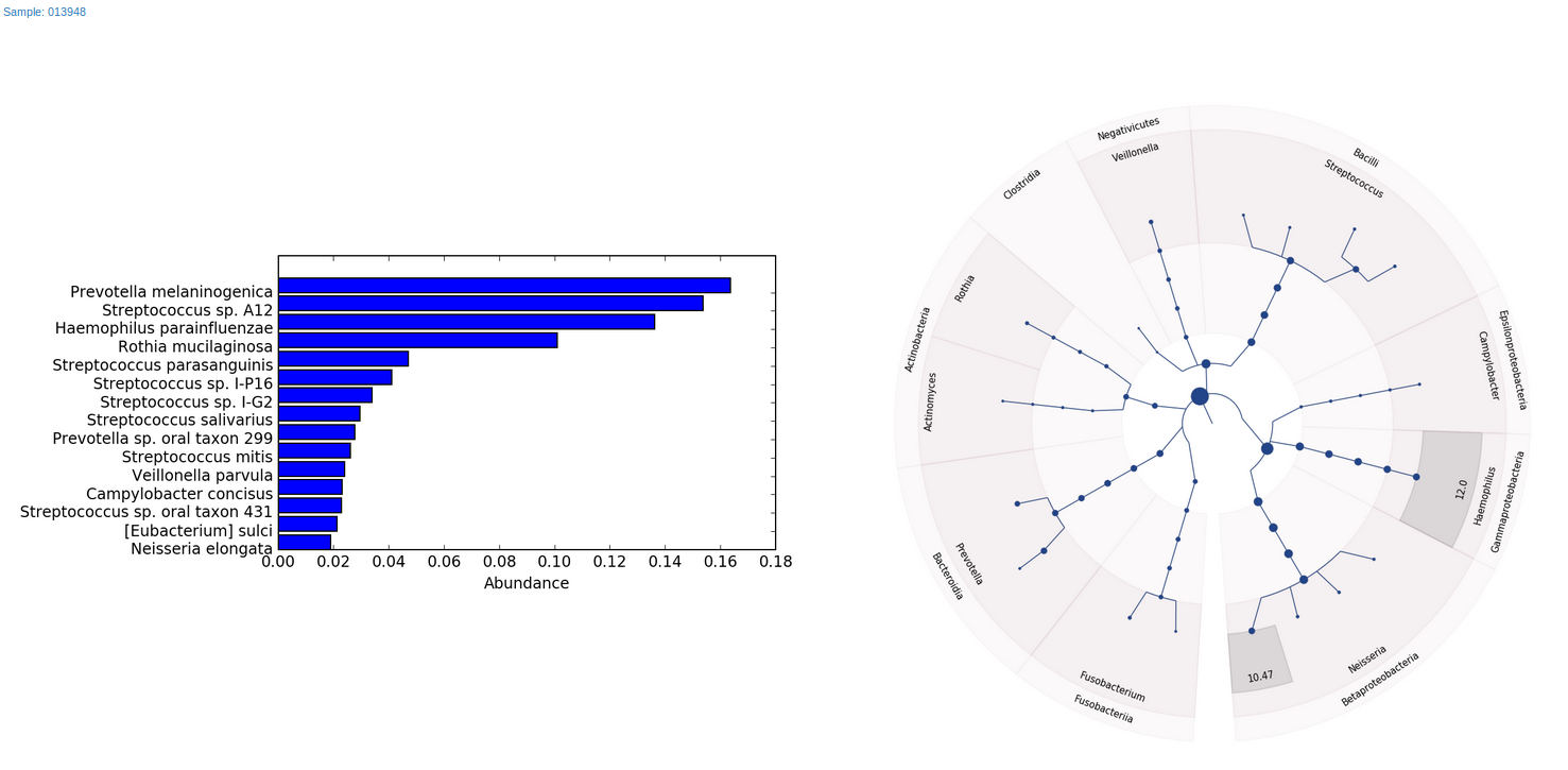
As for final reports, our workflow will generate two HTML files, one with bar charts and Graphlan7 charts for the top abundant species for every sample (Figure 5), and the other with Krona interactive graphs (Figure 1).
Details about Metagenomics WGS analysis – Centrifuge 1.0.3 workflow can be found on its public app page, where you can see the steps it consists of, the complete list of parameters, and more information on how to use it.
Metagenomics WGS analysis – MetaPhlAn 2.0
The other option for profiling metagenomic samples with WGS reads could be by using the Metagenomics WGS analysis – Metaphlan 2.0 workflow, based on MetaPhlAn 2 toolkit 3. This software uses clade-specific marker genes to unambiguously assign reads to microbial clades, up to a species level resolution. MetaPhlAn 2 relies on 1,000,000 unique clade-specific marker genes identified from 17,000 reference genomes (13,500 bacterial and archaeal, 3,500 viral, and 110 eukaryotic). This allows unambiguous taxonomic assignments up to the species-level resolution as well as accurate estimation of organismal relative abundance.
MetaPhlAn has been used during the Human Microbiome Project and, based on our experience, it tends to be up to 25% faster than Centrifuge. That is the reason why we decided to provide the workflow based on this software to our users. However, the classification of reads is based on the pre-built database that could not be customized or extended easily, which may be necessary for some research.
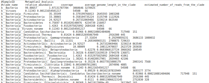
Running Metagenomics WGS analysis – Metaphlan 2.0 requires a FASTQ or FASTA file with whole genome sequencing reads and the metaphlan database. The workflow will produce a report with estimated abundances of taxa per sample (Figure 6).
As in the case of the Centrifuge-based workflow, Metagenomics WGS analysis – Metaphlan 2.0 will also produce final reports with bar charts, Graphlan charts and interactive Krona graphs (Figure 1 and 5).
Details about Metagenomics WGS analysis – Metaphlan 2.0 workflow can be found on its public app page, where you can see the steps it consists of, the complete list of parameters and more information on how to use it.
QIIME2 16S rRNA Metagenomic Profiling
One type of metagenomics analysis is the analysis of sequences coming from marker genes, usually for taxonomic profiling of samples. The most commonly used marker gene is 16S rRNA gene for bacterial and archaeal taxonomic profiling. Compared to WGS, marker-gene sequencing is much cheaper and still sufficient for the identification of species (or other taxa) present in a sample.
QIIME2 16S rRNA Metagenomic Profiling is a workflow based on the QIIME2 toolkit2, used to perform the analysis of microbiome samples using 16S rRNA gene sequences. It is possible to run different analyses by combining tools from QIIME2. We focused on one of the possible solutions, presented in the QIIME2 “Moving pictures” tutorial, which should cover the majority of cases, as it includes importing data into QIIME2 artifact (QZA) format, demultiplexing and quality filtering, OTU picking, taxonomic assignment, and phylogenetic reconstruction of the given samples.
For running this workflow on the Seven Bridges Platform, one needs FASTQ files for one or more samples, the corresponding metadata file and the Classifier in QZA format, a pre-trained Naive Bayes classifier. It is important to train the classifier on a specific dataset of interest, so we recommend using the QIIME2 16S rRNA Feature Classifier Training Workflow to do so. However, if convenient, the other option is to choose the classifier from our Public Repository.
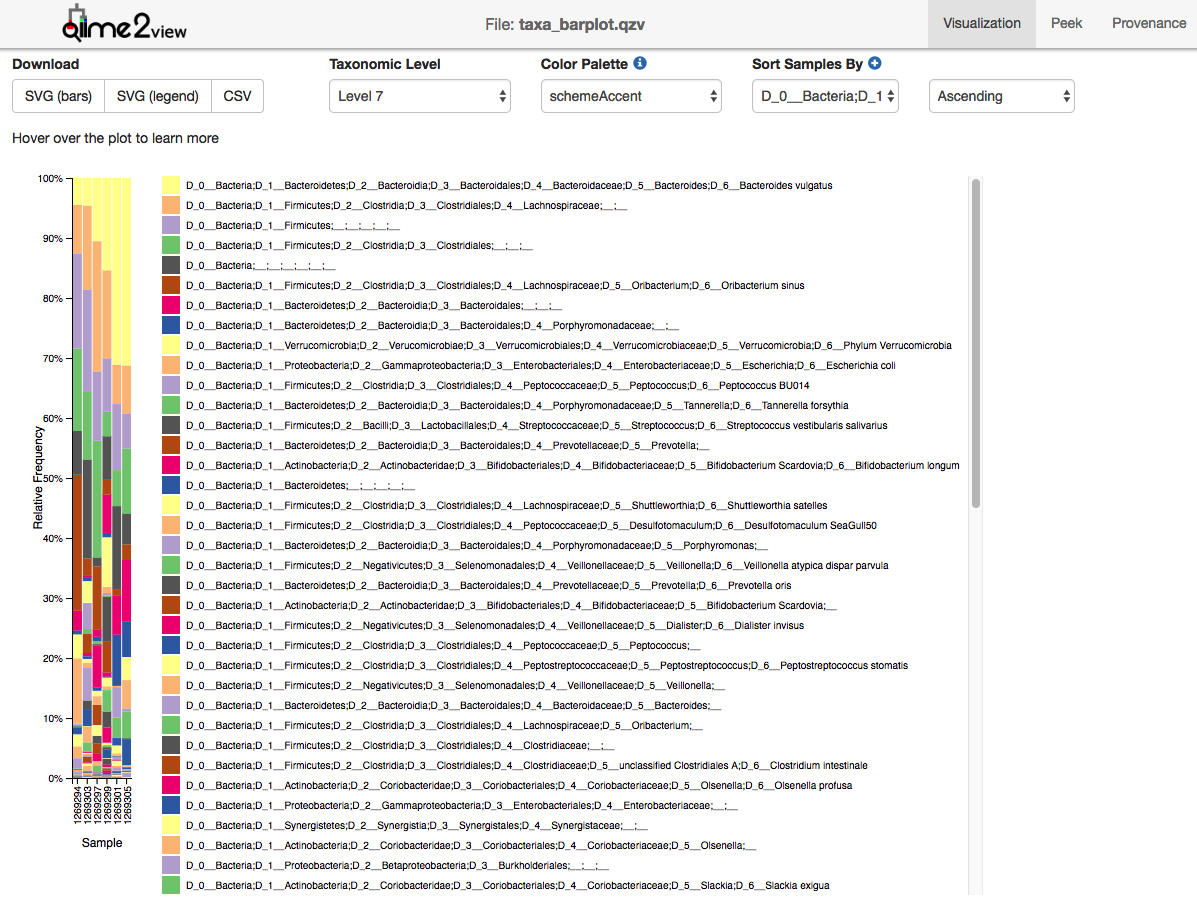
The output from each step of the analyses is given in QIIME2 artifact format, in case there is an interest to analyze it further (QZA files) or view it on the QIIME2 website (visualization QIIME2 artifacts – QZV files). An example of such a visualization file is given in Figure 7.
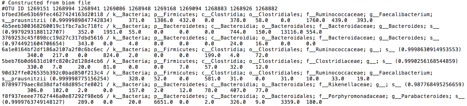
Finally, taxonomic profiles are given in the form of interactive Krona charts, and in TSV format for further differential abundance analysis. The final feature table gives information on each OTU presence in each analyzed sample (Figure 8).
Details about the QIIME2 16S rRNA Metagenomic Profiling workflow can be found on its public app page, where you can see the steps it consists of, the complete list of parameters and more information on how to use it.
Summary
Creation of a taxonomic profile is not the end of research; rather, it is just one of its initial steps. After profiling, further analysis is needed in order to see if there are any differences in profiles obtained from different samples or from different time points, for example. Seven Bridges offers a Jupyter notebook for the differential abundance analysis of metagenomics samples. The code from the notebook can take files from any other project on the Seven Bridges Platform, and is amenable to customization depending on your needs. The same stands for the workflows themselves: if you have specific requirements for the modification or extension of these workflows, you can do so easily (with or without our help) on the Seven Bridges Platform.
References:
- National Research Council (US) Committee on Metagenomics. The New Science of Metagenomics: Revealing the Secrets of Our Microbial Planet. Washington (DC): National Academies Press (US); 2007.
- QIIME2 official web page. QIIME 2 development team; c2016-2020 [accessed 2018 Jun 12]. https://qiime2.org/.
- Segata, N., Waldron, L., Ballarini, A. et al. Metagenomic microbial community profiling using unique clade-specific marker genes. Nature Methods. 2012; 9:811–814. https://doi.org/10.1038/nmeth.2066
- Kim D, Song L, Breitwieser FP, and Salzberg SL. Centrifuge: rapid and sensitive classification of metagenomic sequences. Genome Research. 2016.
- Ondov, Brian D., Nicholas H. Bergman, and Adam M. Phillippy. Interactive metagenomic visualization in a Web browser. BMC bioinformatics. 2011.
- Paulson, Joseph Nathaniel, Mihai Pop, and Hector Corrada Bravo. MetagenomeSeq: Statistical analysis for sparse high-throughput sequencing. Bioconductor package 1.0. 2013.
- GraPhlAn official web page. The Huttenhower Lab: Department of Biostatistics, Harvard T.H. Chan School of Public Health. [accessed 2018 Jun 12]. https://huttenhower.sph.harvard.edu/graphlan.