Highly Customizable Multi-sample Single Cell RNA-Seq Pipeline on the CGC

Written by Nevena Vukojičić, Aleksandar Daničić, Cera Fisher in

Cancer Genomics Cloud

on April 10th, 2023

The reasons and rationale behind single-cell RNA-Seq

“To study human biology, we must know our cells!”  – this is a quote from a paper published a couple of years back [1], where authors of the paper presented early-stage ideas and proofs-of-concept behind The Human Cell Atlas Project, an international collaborative effort aiming to define all human cell types. The goal of this project was to integrate distinctive molecular profiles (such as gene expression) with traditional cellular descriptions (such as location and morphology). One of the key experimental methods utilized for this purpose is single cell RNA-Seq (scRNA-Seq), referring to a class of methods for profiling the transcriptome of individual cells.

Before the emergence of single cell methodologies, transcriptome analyses were initially conducted on large populations of cells or whole tissue samples (or “bulks”). This was due to technical difficulties in isolating a significant enough amount of RNA molecules to be able to  precisely quantify them, from such a small sample as a single cell. Differential transcript expression was first conducted using hybridization-based microarray technology, which was slowly replaced with the next-generation sequencing (NGS) techniques referred to as RNA-Seq. Both of these methods require pooled quantification of gene expressions across all cells in a sample,  and so mask the differences across different cell types. These quantification measures could be quite misleading because gene expressions within small populations of cells will be influenced by the gene expression of the predominant cell populations [2, 3]. Thus, though cells within a sample may actually be quite heterogeneous, the “bulk” methods cannot resolve those differences. 

By contrast, scRNA-Seq analysis allows researchers to explore the whole transcriptome of thousands of individual cells, grouping them into clusters which approximate cell types based on the similarity of transcription profiles. This cellular-level resolution opens up the possibility to analyze transcriptomes of the isolated cell populations, mitigating the problems of bulk methods discussed above. That leads to the identification of rare cell populations, as well as the discovery of novel ones. One of the most widely-used scRNA-Seq applications is the identification of malignant tumor cells within a tumor mass sample. Also, finding differentially expressed genes between different cell subpopulations could lead to the identification of marker genes for specific cell types [2]. 

In this blog post, we first describe the general principles and methods of scRNA-Seq data analysis from the basics of library construction and pre-processing of the input sequencing reads, to the secondary data processing steps needed to normalize and reduce dimensionality across tens of thousands of cells, to the downstream or tertiary analyses used to identify cell populations. We then describe a newly released workflow on the Cancer Genomics Cloud,   Multi-Sample Clustering and Gene Marker Identification with Seurat, an easily deployable pipeline for the downstream analysis of scRNA-seq experiments. We demonstrate the capabilities of this workflow using two previously published datasets of pancreatic cells [12, 13].

The basic steps of scRNA-Seq

Typical scRNA-Seq analysis flow can be divided into three phases – pre-processing, data processing and downstream analysis, shown in Figure 1 [3].

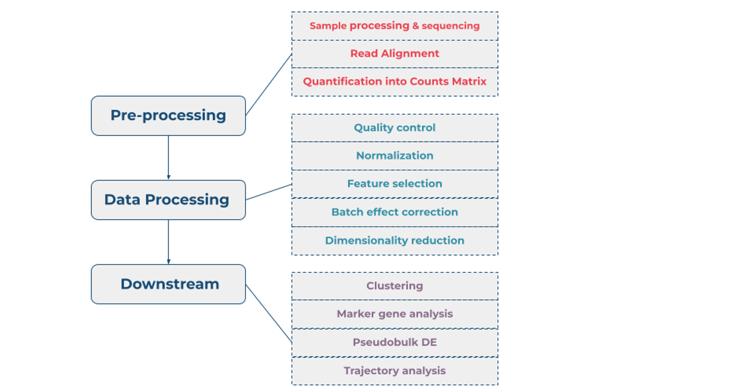
Pre-processing

The first step in obtaining transcriptome information from an individual cell is the isolation of viable, single cells from the tissue of interest. Isolated cells are lysed to allow capture of RNA molecules. The majority of single cell protocols analyze polyadenylated mRNA molecules, because the analysis of non-coding RNA fraction represents significant challenge [2]. The construction of the sequencing libraries for scRNA-seq is similar to that used for bulk RNA-Seq methods, except that steps must be taken to isolate cells prior to RNA extraction and capture each cell’s RNA individually for barcoding [2]. After capturing, RNA is converted to complementary DNA (cDNA) by a reverse transcriptase. cDNAs are then exponentially amplified by PCR or, linearly by in vitro transcription followed by another round of reverse transcription. After library construction, sequence libraries are pooled and sequenced by NGS. The analysis and interpretation of the sequencing data is performed using tools and pipelines similar to those used for bulk RNA-Seq [2]. 

Alignment is the first and one of the most critical steps of computational scRNA-seq analysis. In general, the aim of the alignment step is to find the original transcriptomic location of the experimentally obtained sequencing reads. The choice of the alignment tool and its algorithm (splice-aware or pseudoalignment) directly affects all subsequent downstream analysis steps and biological findings. The second step is the successful quantification of a sequencing read to a specific genomic location, represented by a count matrix. Alignment and quantification steps are often performed together, and the most popular tools used for this purpose are Cell Ranger counts, Salmon Alevin, Kallisto BUStools Workflow, zUMIs, Single-Cell Smart-seq2 Workflow v3.0.0, and STARsolo, all of which (save CellRanger) are available in the Public Apps gallery on the CGC Platform. Obtained gene-cell count matrices are used as inputs for further data processing analyses [2, 3].

Data processing

Before further analyses, quality control of scRNA-seq data should be undertaken. In this step, any poor-quality data, which could result from a variety of causes [2,3], is excluded from subsequent analysis. Currently, there is no consensus on exact filtering strategies, but commonly used criteria include relative library size, number of detected genes and fraction of reads mapping to mitochondria-encoded genes or synthetic spike-in RNAs [2]. Next step is normalization, a crucial part of the analysis flow, addressing limitations presented by technical noise or bias. Over the years, several normalization methods have been developed, ranging from variations of bulk sequencing methods to entirely new approaches designed specifically for single-cell studies [4]. After normalization come analysis steps such as clustering and dimensionality reduction. These methods involve comparing cells based on the similarity of their gene expression profiles, but not all genes are reliable – some genes may have uninformative expression patterns, particularly lowly expressed genes. Therefore, a feature selection step helps to select the most biologically meaningful genes, while removing the ones that contain random noise. The simplest approach here is to consider the most variable genes based on their expression across the population [3]. 

In some cases, an additional step is needed – batch effect correction. RNA-seq in general is prey to well-known batch-effect problems, and scRNA-seq may be particularly sensitive. This applies if researchers have multiple datasets they wish to analyze together, such as serial runs of the same libraries, or even separate experiments that originate from the same kind of biological samples. The batch effect correction step controls for technical variance when combining cells of different batches or from different studies. Multiple batch effect removal algorithms have been developed to date, usually based on supervised or unsupervised detection of mutual nearest neighbors (MNNs) in the high-dimensional expression space [5]. 

Finally, scRNA-seq data is highly dimensional; e.g., a single dataset may be a matrix of 10,000+ samples across 187,000 transcripts. Therefore, a dimensionality reduction is a necessary step to visualize and interpret the results. Principal component analysis (PCA) is a mathematical algorithm that reduces the dimensionality of data, and is a basic and widely used tool in scRNA-seq data processing. Since the development of RNA-seq technology, this linear dimension-reduction method has been favored by researchers. In addition, there are non-linear methods such as uniform manifold approximation and projection (UMAP) and t-distributed stochastic neighbor embedding (t-SNE) to reduce dimension, that are also widely used in scRNA-seq analysis [2].

Downstream analysis 

After data processing, a few methods that we group into downstream analysis are used to extract biological insights and describe the underlying biological systems. These descriptions are obtained by fitting interpretable models to the data. Clustering is typically the first step of a downstream analysis, because it allows us to explore the data and summarize complex scRNA-seq data into a digestible format. Clusters are obtained by grouping cells based on the similarity of their gene expression profiles and allow us to infer the identity of member cells [6]. We can zoom in and out by changing the resolution of the clustering parameters, and we can experiment with different clustering algorithms to obtain alternative perspectives of the data. The most commonly used clustering algorithms are graph-based clustering, vector quantization with k-means, and hierarchical clustering. Graph-based clustering (precisely, Louvain algorithm) is used in the Seurat R package, as a method that constructs a graph using cells as nodes, where cells with similar transcriptomes are connected by edges. The Louvain algorithm then clusters cells by trying to divide the graph so that the modularity is maximized. This method outperforms others when dealing with large datasets in terms of speed and accuracy [3, 7]. 

To interpret the clustering results, we identify the genes that drive separation between the clusters. These marker genes facilitate assigning biological meaning to each cluster. The most straightforward approach to detect marker genes is testing for differential expression between all clusters. If a gene is strongly differentially expressed between clusters, it is likely to have driven the separation of cells in the clustering algorithm [3].

Identification of marker genes has great importance in cell cluster annotation. This remains one of the key challenges of scRNA-seq research. A possible solution could come from the generation of the data itself, as the more data is accumulated, the more unknown clusters can be matched with previously known clusters [8]. Usually, there are two ways of annotating cell clusters – manually and automatically. Identification of clusters can be performed manually using available databases that contain marker genes for various cell types. Automated cell type annotation is reference-based,and uses tools developed by the community for automatically annotating cells by comparing new data with existing references [9].

Another type of scRNA-Seq downstream analysis is differential gene expression analysis (DGE) between conditions with biological replicates. DGE between conditions can be done separately for each cell type, enabling direct interpretation of the underlying differences in biological pathways and mechanisms [10]. To make analysis computationally tractable, DGE testing is performed on pseudobulk expression profiles, generated by summing counts together for all cells with the same combination of label and sample. This leverages the resolution offered by single-cell technologies to define the labels, and combines it with the statistical rigor of existing methods for DGE analyses involving a small number of samples [3].

Also, scRNA-Seq can facilitate the prediction of a theoretical lineage trajectory along a pseudotime scale to uncover the molecular programs that drive developmental processes. This is because it can reveal the gene expression profiles of both the steady and transitioning states of captured cells. Assuming that the captured cells are not only at the start or end of the transition but also in intermediate phases of development, one could create a lineage trajectory map along a pseudotime scale and subsequently identify candidate factors associated with the transitional populations by removing biases generated by other cell types [11].

Multi-Sample Clustering and Gene Marker Identification workflow

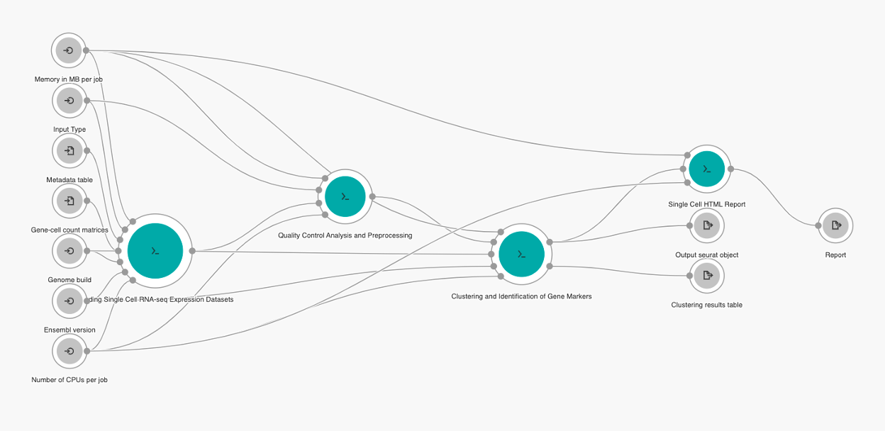
In this blog, we will highlight our new scRNA-Seq workflow, Multi-Sample Clustering and Gene Marker Identification workflow with Seurat 4.1.0, which covers all the data processing steps: quality control, normalization, feature selection, batch effect correction and dimensionality reduction, as well as clustering and gene marker identification as downstream analyses. This workflow is the latest Seven Bridges solution for processing multiple input scRNA-seq datasets, based on the latest version of the Seurat package (v4.1.0), offering multiple options for each of the standard scRNA-seq analysis steps. Our solution supports gene-cell count matrices generated by several commonly used quantifiers (e.g., CellRanger, Salmon Alevin, Kallisto BUStools, STAR) coming from single or multiple single-cell datasets from different batches, as well as single or multiple samples combined in a SingleCellExperiment R object. The outputs include a detailed HTML report, containing quality metric and clustering result plots, a table with all detected cluster-specific gene markers, and the resulting Seurat R object. 

We demonstrate the versatility of the pipeline with several implemented options to choose from at each of the analysis steps: filtering, normalization, batch effect correction, and differential expression performed after the clustering step. The solution is based on Seurat v4.1.0, but other R packages and methods are used where certain  steps cannot be processed using Seurat, or when the Seurat solution is much slower. Quality control can be performed manually or automatically using several options for normalization (LogNormalize, Deconvolution, SCnorm and Linnorm) and for batch effect correction (Seurat and Harmony). For clustering, the pipeline uses Seurat’s graph-based approach, with options for different clustering resolutions. After performing identification of the gene markers for each cluster, a researcher can test differential expression using various options including Wilcoxon Rank Sum, logistic regression, negative binomial and poisson distributed generalized linear models, likelihood-ratio tests, ROC analysis, MAST, and DESeq2.

Pipeline Design

The pipeline consists of the following tools (Figure 2):

• Loading Single Cell RNA-seq Expression Datasets; 
• Quality Control and Preprocessing; 
• Clustering and Identification of Gene Markers; and
• Single Cell HTML Report generation tool

Validation of the solution

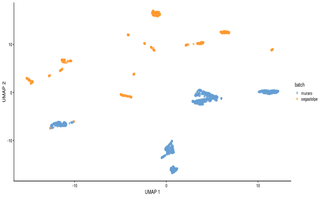
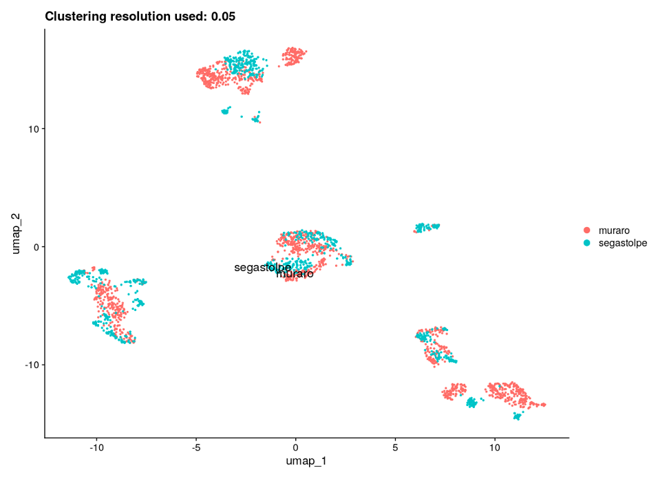
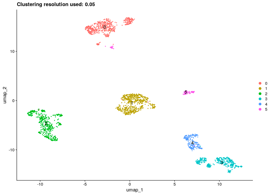
To demonstrate the workflow’s capabilities and at the same time to validate it, a SingleCellExperiment object was used as an input, containing previously merged Muraro [12] and Segerstolpe [13] datasets of pancreatic cells. Both datasets were  first preprocessed in a way to keep specific pancreatic cell types (alpha, beta, gamma, ductal and acinar cells) from healthy individuals. The merged datasets were then processed with the Multi-Sample Clustering and Gene Marker Identification with Seurat 4.1.0 pipeline with default settings. The effects of the batch correction step, performed using Harmony package, are shown in Figure 3.

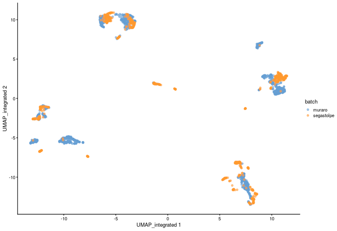
After performing the clustering and gene marker identification steps for several clustering resolutions ranging from 0.05 to 0.6, we chose 0.05 as the most suitable resolution based on the UMAP plots when the cell types are presented and other results obtained with the Multi-Sample Clustering and Gene Marker Identification with Seurat 4.1.0 pipeline. In addition, the adjusted rand index, a metric which measures the similarity between two clusterings (0-1), was calculated; the highest value of 0.53 was obtained for clustering resolution of 0.05. UMAP plots for the chosen clustering resolution are shown in Figure 4, with color-space partitioned by dataset (A), cell type (B), and automated clusters (C).

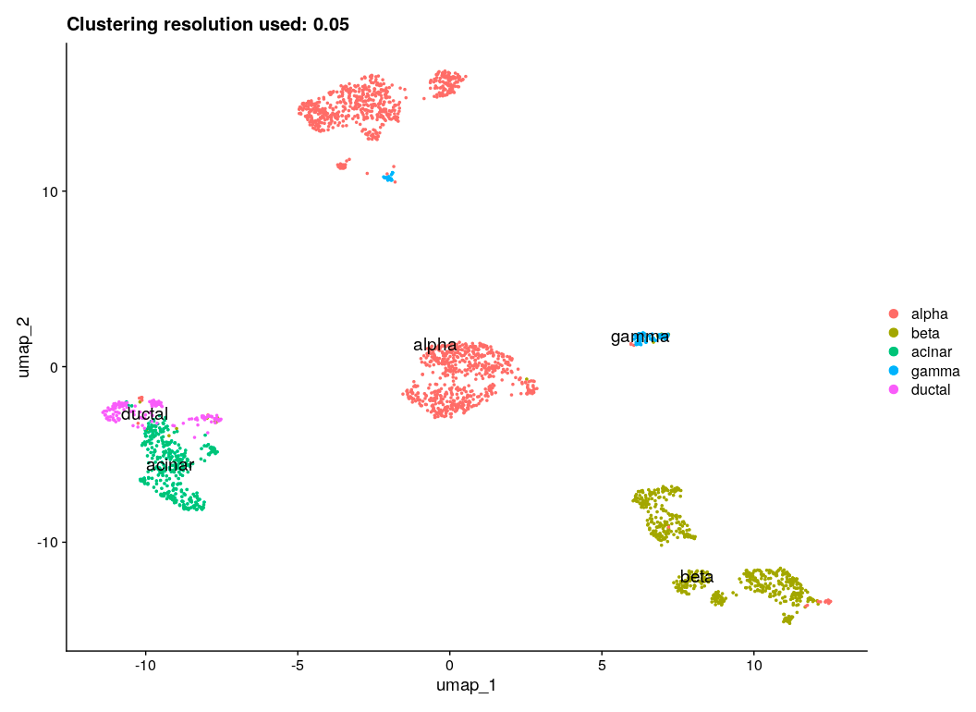
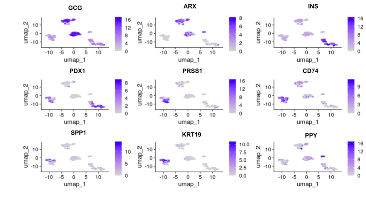
Finally, to validate results and connect identified gene markers to specific cell types/clusters, we found known gene markers for each of the pancreatic cell types and produced corresponding feature plots (Figure 5). All of the specific cell type marker genes matched corresponding clusters.

Performance benchmarking

Table 1 below summarizes the computational resources we found work well to run the Multi-Sample Clustering and Gene Marker Identification with Seurat 4.1.0 workflow via AWS on different datasets using the Seven Bridges cloud environment. This table provides typical values you can expect when running this workflow for datasets of different numbers of cells, from 1-160k cells per dataset, and using 1 or 2 clustering resolutions. It shows us that after dataset size, the number of different clustering resolutions specified is the most important factor influencing the duration and cost of the workflow. Other dataset qualities, including sample complexity and target gene sequences, can also influence duration. 

 

# of cells	# of resolutions	Duration	Cost	Instance (AWS)
1.2 k	2	6min	0.06$	c4.2xlarge
4.6 k	2	8min	0.07$	c4.2xlarge
8.7 k	2	15min	0.14$	c4.2xlarge
11.7 k	2	34min	0.31$	c4.2xlarge
1.2k + 4.6k + 8.7k + 11.7k	2	25min	0.23$	c4.2xlarge
30k	2	15min	0.14$	c4.2xlarge
50k	2	43min	1.21$	c5.9xlarge
61k	1	2h59min	5$	c5.9xlarge
61k	2	6h43min	11.23$	c5.9xlarge
84k	1	2h3min	3.44$	c5.9xlarge
84k	2	4h7min	6.89$	c5.9xlarge
160k	1	10h 5min	16.87$	c5.9xlarge
160k	2	21h 35min	36.10$	c5.9xlarge

Table 1. Performance Benchmarking for the Multi-sample Clustering and Gene Marker Identification with Seurat 4.1.0

The prices listed vary based on the selection of on-demand or spot instances. See the Spot Instance Advisor for more information regarding on-demand versus spot instances.

In conclusion

Advances in single cell sequencing technology allow increasingly accurate and efficient analyses, with more and more researchers incorporating it into their work. It is expected that scRNA-Seq will continue to play a major role in the field of transcriptomics. Further development of scRNA-Seq techniques will undoubtedly improve our understanding of tumor biology and highlight promising drug targets. As the field continues to grow, the CGC’s cloud-based computation infrastructure, along with numerous available cancer datasets and easy-to-use single-cell data processing workflows as the one presented in this blog,  will be instrumental in helping researchers distill new knowledge of cancer and its disease processes.

References

1. Regev, A., et al. “Human Cell Atlas Meeting Participants: The human cell atlas.” Elife 6.
2. Haque, A., et al. “A practical guide to single-cell RNA-sequencing for biomedical research and clinical applications.” Genome Med. (2017): 75.
3. Amezquita, Robert A., et al. “Orchestrating single-cell analysis with Bioconductor.” Nature methods 17.2 (2020): 137-145.
4. Lytal, Nicholas, Di Ran, and Lingling An. “Normalization methods on single-cell RNA-seq data: an empirical survey.” Frontiers in genetics 11 (2020): 41.
5. Haghverdi, Laleh, et al. “Batch effects in single-cell RNA-sequencing data are corrected by matching mutual nearest neighbors.” Nature biotechnology 36.5 (2018): 421-427.
6. Luecken, Malte D., and Fabian J. Theis. “Current best practices in single‐cell RNA‐seq analysis: a tutorial.” Molecular systems biology 15.6 (2019): e8746.
7. Kiselev, Vladimir Yu, Tallulah S. Andrews, and Martin Hemberg. “Challenges in unsupervised clustering of single-cell RNA-seq data.” Nature Reviews Genetics 20.5 (2019): 273-282.
8. Adil, Asif, et al. “Single-Cell transcriptomics: current methods and challenges in data acquisition and analysis.” Frontiers in Neuroscience 15 (2021): 591122.
9. Web resources for cell type annotation – 10x Genomics
10. Differential Gene Expression Analysis in scRNA-seq Data between Conditions with Biological Replicates – 10x Genomics
11. Wu, Szu-Hsien Sam, Ji-Hyun Lee, and Bon-Kyoung Koo. “Lineage tracing: computational reconstruction goes beyond the limit of imaging.” Molecules and cells 42.2 (2019): 104.
12. Muraro, Mauro J., et al. “A single-cell transcriptome atlas of the human pancreas.” Cell systems 3.4 (2016): 385-394.
13. Segerstolpe, Åsa, et al. “Single-cell transcriptome profiling of human pancreatic islets in health and type 2 diabetes.” Cell metabolism 24.4 (2016): 593-607.